|
Start
Excel
Text
& Numbers
Column
Widths
Selecting
Rows
Auto-Fill
Format
Numbers
Formulas
Absolute
& Relative References
Functions
Borders
Cell
Comments
Multiple
Sheets
Charts
Multimedia
Tools
Sorting
Protection
|
Spreadsheets
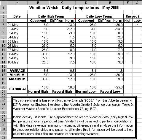
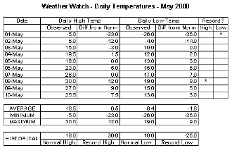
In this tutorial we will create a sample spreadsheet. The finished
product is displayed below:
- Launch Excel. (Usually on Windows computers you can click
on the Windows Start menu / Programs / Microsoft Excel.
Check with your instructor if you are not sure how to launch Excel
on the computer you are using.)
  
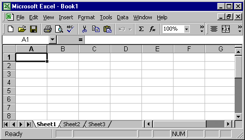
- A blank Excel spreadsheet appears.

- A computerized spreadsheet can make it easier to perform calculations
and experiment with numbers. With a spreadsheet you can type in equations
once and then change the data many times with the computer automatically
re-doing the calculations for you (unlike using a hand-held calculator
or working out equations by hand!).
A spreadsheet is a grid of columns and rows - the computer equivalent
of a paper ledger sheet. The intersection of each row and column
is called a "cell". Cells are referred to by their column letter
and row number. e.g. The cell highlighted in the picture is called
cell A1, the cell to the right of it is B1, the cell
below it is A2, etc.
At any time, you can start a new spreadsheet by clicking on the
Excel File menu and selecting New, or open an existing
file by selecting File / Open.
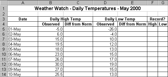
- First we will explain how to enter and format some text and numbers
in the first few rows of the spreadsheet as shown below:

- To enter information into a spreadsheet, you simply click the mouse
on the cell where you want data to appear, and then type.
- Click your mouse in Cell A1 and type "Weather Watch - Daily Weather
Information - May 2000", then press the Enter key. Notice that
if a cell is not wide enough to hold the text you type, the text simply
spills into the adjoining cells to the right.
- To give the text bold styling, click on Cell A1 again, then click
the Bold button
 at the top of the screen (same as word processing, right?). at the top of the screen (same as word processing, right?).
- Still on Cell A1, increase its font size by clicking on the
Font Size drop-down list
 (the example is set to 12 point). (the example is set to 12 point).
- Now, how do we get the text in Cell A1 to appear centered between
columns A to G?. Simple in Excel. First, highlight cells A1 through
G1 (click and hold the mouse button down on A1 then drag to the right
to G1 - or click on A1, then move the mouse to G1, hold the shift
key down and click the mouse). Second, click the Merge and Center
button
 . Cells A1 through G1 are now
merged (treated as if they were one cell) and the text is now centered
within this larger cell area. . Cells A1 through G1 are now
merged (treated as if they were one cell) and the text is now centered
within this larger cell area.
- Now, type the text that you see in the cells in rows 3 and 4 in
the above example (Note: "Daily High Temp" goes in B3, "Daily Low
Temp" goes in D3, and "Record?" goes in F3). Without the formatting
applied in our example, your data will probably look something like:

- There are several little formatting operations we can do to make
the titles in rows 3 and 4 look a little nicer.
- First of all, we need to widen columns C and E so that the
text entered in cells C4 and E4 is completely visible. To widen column
C, place the mouse on the boundary between columns C and D at the
top where the column names are. The cursor should turn to a double
arrow as shown in the picture below. Click, hold, and drag the mouse
to the right until column C is wide enough to display all of the text
in Cell C4 (i.e. "Diff from Norm"). Similarly, widen column E.

- How would you narrow a column? You guessed it - do the same
thing as above except drag left instead of right. See if you can make
columns F and G narrower. Another trick: instead of dragging the cursor,
just double-click it for an auto-fit (automatically adjust
to the widest entry in the column).
- Second, we want all of the text in rows 3 and 4 to be in Bold
style. This can be done in one fell swoop - no need to do each cell
one at a time. One quick method is to select all of rows 3 and 4 -
to do this place the cursor over the number 3 (which indicates row
3) on the far left, click and hold the mouse button, then drag the
mouse down to the number 4 below it, and finally release the mouse
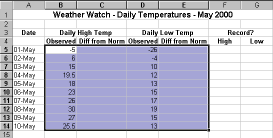
button (all of rows 3 and 4 should be highlighted as shown below).
Then, of course, click the Bold button
 . .

- While you have Rows 3 and 4 highlighted, also click on the Center
button
 to
make all of the text centered within each cell in those rows. to
make all of the text centered within each cell in those rows.
- Finally, do that Merge and Center
 operation on cells B3 and C3,
then again on cells D3 and E3, and again on cells F3 and G3. operation on cells B3 and C3,
then again on cells D3 and E3, and again on cells F3 and G3.
- Now, let's enter those dates that belong in column A. Click
on cell A5 and type "01-May".
- Here's a trick to help you quickly enter the dates "02-May" to "10-May":
- Click on cell A5, then position the mouse in the bottom right
of the cell so that the cursor turns to a small black plus sign,
as shown below.
- With the cursor as such, click, hold and drag the mouse down
to cell A14, and then release the mouse.
- Excel automatically copies the date and increments by one day
for each cell going down, giving you the series 01-May, 02-May,
... , 10-May.

- Note: Advanced options on creating such auto-fill series
are available with the menu command Edit / Fill / Series.
Now, see if you can add the additional text and numbers in cells A16
to E21 shown below. The text labels ("AVERAGE" ... "Record Low") should
all be Bold and Centered. The numbers in cells B20 to
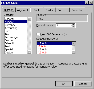
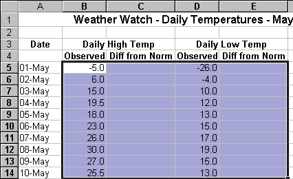
E20 should be formatted with one decimal place. Cells A20/21
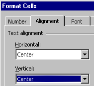
are a little tricky: "HISTORICAL" should be typed into cell A20, then
Merge and Center cells A20 and A21, then click on Format /
Cells / Alignment / Vertical: Center.


Now for the real power of spreadsheets - formulas! (If you're not going
to use formulas in a spreadsheet, you're just as well off to simply
use a word processor and create a table to format information as we've
done so far with the text and numbers above.)
- In Column C, we want to insert equations which will calculate
the difference between the observed daily high temperatures (from
column B) and the historical normal high (from cell B20).
- In cell C5 type the following (include the =, all Excel formulas
must start with this symbol, the reason for the $ will become apparent
later):
=B5-$B$20
- Press the Enter key when you are done typing the formula.
- If you typed in the same data as our example, you should see the
result -23.0 displayed in cell C5.
- A similar formula must be placed in cells C6 to C14, but you won't
have to retype it! We can copy formulas using the same technique
used earlier to copy the dates in column A.
- Click on cell C5, then position the mouse in the bottom right of
the cell so that the cursor turns to a small black plus sign. With
the cursor as such, click, hold and drag the mouse down to cell C14,
and then release the mouse. Excel automatically copies the formula
and increments the row number from the original B5 cell reference
for each cell going down. Notice, however, that it didn't alter
the $B$20 cell reference - but that is good because every one of these
difference equations must refer to that exact cell (B20). B5 is an
example of a relative cell reference (it is automatically adjusted
when copying a formula to other cells), while $B$20 is an example
of an absolute cell reference (it is left as is when copying
to other cells).
- See if you can figure out what formula should be typed into cell
E5 to calculate the difference between the observed daily low temperatures
(from column D) and the historical normal low (from cell D20). Copy
the formula to cells E6 to E14.
- Here's one further subtle detail - a cell reference can be partially
relative and partially absolute. We could have typed =B5-B$20
into cell C5 and the copying down to the other cells would still have
worked fine. B$20 means that the column part (B) is relative and the
row part ($20) is absolute. See what happens if you click on cell
C5 (containing this new version of the formula), then click on Edit
/ Copy, then click on cell E5, and then click on Edit / Paste.
You should see =D5-D$20 in cell E5. With a good understanding
of how relative and absolute cell references work, we can really avoid
unnecessary typing of formulas - we can use auto-filling or copy/paste
all over the place!
- In row 16, we want to create equations which will automatically
calculate the average of the values in columns B to E.
- In cell B16 type:
=AVERAGE(B5:B14)
- AVERAGE is a built-in Excel function which automatically
calculates the average of a set of values - much easier than typing
in an equation such as (B5+B6 ... +B14) / 10. B5:B14 is called a range
of cells, and refers to the whole block of cells from B5 to B14
inclusive.
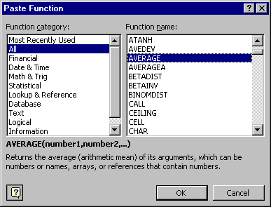
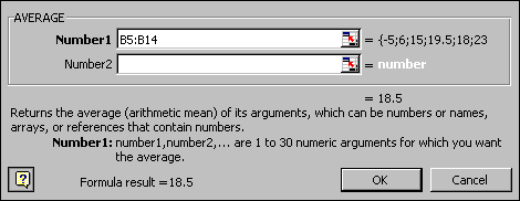
- There is a second way to insert a function into a cell. Click on
the cell (in this case B16), then click on Insert / Function
- this opens the Paste Function window. Choose the desired
function (in this case AVERAGE), then click OK. This opens
another window which lets you indicate which cells the function should
operate on. To the right of Number 1, type the desired range
of cells (or you can even indicate the cells with the mouse by highlighting
the blocks of cells directly on the spreadsheet). Click OK again and
the correct formula should appear on the spreadsheet.


- A similar formula must be placed in cells C16 to E16, but again,
you won't have to retype it! We can copy formulas using the
same technique used earlier.
- Click on cell B16, then position the mouse in the bottom right of
the cell so that the cursor turns to a small black plus sign. With
the cursor as such, click, hold and drag the mouse (to the right this
time) to cell E16, and then release the mouse. Excel automatically
copies the formula and increments the column letters from the original
B5:B14 cell range reference for each cell going across.
- In rows 17 and 18, we would like to display the minimum and
maximum of the values in columns B to E. See if you can use
the function MIN to create the equations for row 17 (cells
B17 to E17) and the function MAX to create the equations for
row 18 (cells B18 to E18). The correct formulas are shown below.

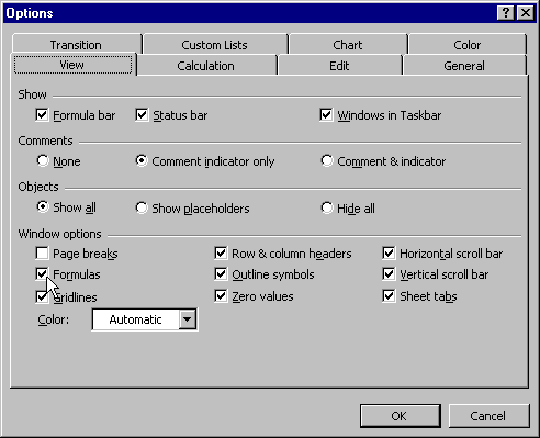
Note: To change the spreadsheet view as shown above (see actual formulas
in the cells instead of their numeric results) - on the Tools
menu, click Options, click the View tab, then place
a checkmark beside Formulas, then click OK.

- In column F we want to insert formulas which flag whether or not
a record high temperature was reached on any of the days.
- In cell F5 type the formula shown below, then copy it to cells F6
to F14:
=IF(B5>=$C$20,"*","")
Note: Some Macintosh versions of Excel require a semicolon (;)
instead of a comma (,) to separate the parts of the IF function; if
you use a comma you get a message stating that there is a syntax error
in your formula.
- The above formula makes use of the IF function to allow us
to compare one value to another and then set the cell contents based
on the result of the comparison using the syntax:
=IF(logical_test,value_if_true,value_if_false)
The logical_test we are using is B5>=$C$20 (i.e. is
the observed daily high temperature greater then or equal to the record
high).
The value_if_true we are using is "*" (i.e. put a * in the
cell if the logical test is true).
The value_if_false we are using is "" (i.e. put nothing (an
empty text string) in the cell if the logical test is false; if we
didn't specify the value_if_false, Excel would put the word "FALSE"
into the cell, which would look a little messy).
- Similarly, to flag new record low temperatures, in cell G5 type
the formula shown below, then copy it to cells G6 to G14:
=IF(D5<=$E$20, "*","")
- If you have entered the data and formulas as per our sample, a "*"
should appear in two cells: G5 (01-May had a record low) and F12 (08-May
had a record high)
Another formatting feature which can improve the readability of a spreadsheet
is to add borders around cells. This is especially useful if you are
going to print your spreadsheet because, by default in Excel, the light
gray cell gridlines don't appear when you print a spreadsheet document.
- To set borders, first select the cells on which you want to put
borders.
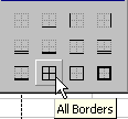
- Then click the Borders button on the toolbar at the top of
the screen.

- Select a border style from the options that are displayed. In the
example below, the All Borders options is selected - this places
a single line around all sides of all of the selected cells.

- In the sample spreadsheet displayed at the beginning of this tutorial,
you will notice borders around various parts of the spreadsheet -
this helps to separate it into logical sections.
- Highlight cells A3 to G14 (the daily temperatures area), click
on the Border button as shown above, and select the All
Borders style.
- Do the same with the area A16 to E18 (averages, maximums, and
minimums) and the area A20 to E21 (historical data).
- The following print preview snapshot shows what would appear
on a printout with the borders applied as indicated above:

- Note 1: An alternative way to set borders (which gives you many
more options) is to select the cells, then click on the Format
menu, then select Cells, then click the Border tab.
- Note 2: If you don't want to bother adding borders you can get the
gridlines to appear when you print a spreadsheet - on the File
menu, click Page Setup, and then click the Sheet tab.
Select the Gridlines check box. Warning - this gives you ALL
of the gridlines on ALL of the cells on a page, and can make printing
very slow.
- Cell comments are additional explanatory notes which you
can attach to a cell in a spreadsheet.
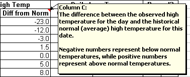
- Cell C4 in the sample spreadsheet has a cell comment associated
with it, as indicated by the small red triangle in the upper right
corner of the cell.
- To view the comment, rest the pointer over the cell. A text box
will appear, as shown below .

- To add a comment to a cell, click the cell to which you want to
add the comment.
- On the Insert menu, click Comment.
- In the box, type the comment text.
- When you finish typing the text, click outside the comment box.
- To edit an existing cell comment, click the cell with the comment
you want to edit.
- On the Insert menu, click Edit Comment.
An Excel spreadsheet file is technically referred to as a Workbook,
and can contain several individual spreadsheets called Worksheets.
This feature allows you to organize various kinds of related information
in a single Excel file. Up until now in this tutorial, we have been
working with just one worksheet, the default first sheet named Sheet1
which is displayed when you start a new Excel spreadsheet file.
- At the bottom of the Excel screen are Sheet tabs.

- To move from sheet to sheet, click the sheet tabs. If you
click on Sheet2 or Sheet3 right now you will see that they are separate
blank spreadsheets.
- If you are using a large number of sheets, you can use the tab
scrolling buttons to the left of the sheet tabs to move the tabs
display left or right.
- To rename a sheet, double-click the sheet name on the sheet
tab, then type a new name over the current name.
- To delete a sheet, first select the sheet you want to delete,
then on the Edit menu, click Delete Sheet.
- In the sample file you are creating, try renaming Sheet1 to Main
and deleting Sheet3. Your sheet tabs should now look like:

- There are numerous other operations available for managing worksheets
with an Excel workbook (e.g. move or copy sheets). For further information
read the Microsoft Excel Help / Contents / Working with Workbooks
and Worksheets / Managing Worksheets.
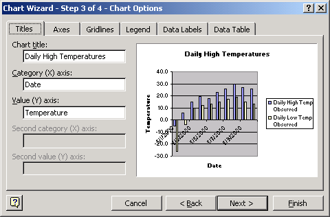
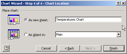
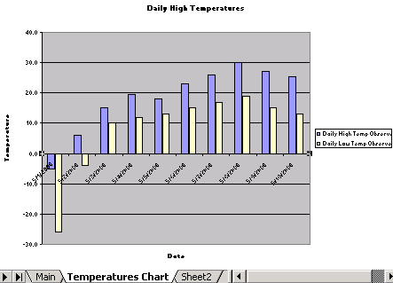
In this section, we will add a chart to our sample spreadsheet workbook
and store it on a new worksheet. The chart will provide a graphic representation
of the high and low temperature data in the spreadsheet.
- Select the cells that contain the data that you want
to appear in the chart. If you want column and row labels to appear
in the chart, include the cells that contain them in the selection.
In our sample, we should highlight the block of cells A3 to
E14.
- Click the Chart Wizard button (or on the Insert
menu click Chart).
- A window entitled Chart Wizard - Step 1 of 4 - Chart
Type is displayed. There are many options available, but for our
example we will just accept the default Column chart type displayed.
Click the Next button.
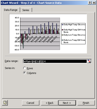
- Step 2 of the chart wizard appears. The Data Range
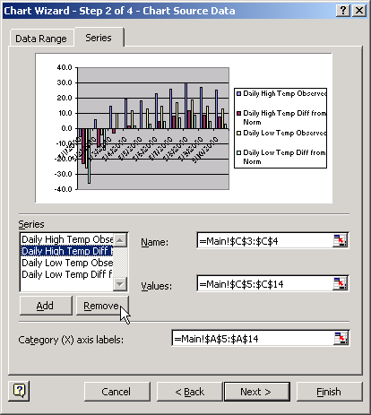
tab should appear as shown on the left below. Click on the Series
tab to see some other options as shown on the right below. We will
simplify the chart by only including the two Observed Temperature
columns (not the two "diff" columns). Currently four series of data
are listed in the Series box near the center left. Click on "Daily
High Temp Diff ..." and click on the Remove button. Similarly, remove
"Daily Low Temp Diff ...", then click the Next button.


Many of the same commands for working with multimedia that are available
in other Microsoft Office programs (Word, PowerPoint) are also available
in Excel.
- For example, you can use familiar Drawing Tools in Excel
by displaying the Drawing Toolbar - click on the View
menu, then click Toolbars, then select Drawing.

- In our sample spreadsheet, we used a drawing tool to create a large
text box near the bottom of the spreadsheet as follows.
- Click on the Text Box
 button in the drawing toolbar. button in the drawing toolbar.
- Put the mouse over the blank area below the occupied area of
the spreadsheet
- The cursor will change to a narrow down-arrow (as shown on the
left below). Click, hold, drag, and release the mouse to form
a rectangle on the sheet. Then you can type into the text box
created for you (as shown on the right below).
 
- For further information on the following operations, please see
our PowerPoint
tutorial.
- To add a picture from an image file, click on Insert / Picture
/ From File.
- To create a WordArt graphic out of text, click on the
Insert / Picture / WordArt.
- To insert Clip Art, click on Insert / Picture / Clip
Art.
- To create a bar or pie chart, on Insert / Chart.
- To insert an organization chart, click on Insert /
Picture / Organization Chart.
- To insert other objects (e.g. movies, other documents), click
on Insert / Object.
The data in a spreadsheet is sometimes more meaningful if it appears
in a certain order. With the sorting tools in Excel, you can rearrange
rows of data according to the contents of one or more columns. As an
example of sorting, we will create a second copy of the Main worksheet
and sort the data on the new sheet in a different order (you don't have
to create a copy of data to sort it, we are just doing it for comparison
sake).
To create a copy of the Main sheet:
- Select the Main sheet (formerly called Sheet1).
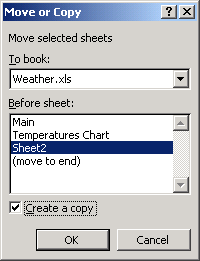
- On the Edit menu, click Move or Copy Sheet (or right-click
the Main sheet tab and select Move or Copy).
- The Move or Copy window appears.
- Put a check mark beside Create a Copy and under Before
sheet: indicate where the new sheet should be positioned, similar
to the example below.

-
Note: You can also use drag-and-drop to copy a
sheet. Hold down the Ctrl key, drag the selected sheet tab
to its new position among the sheet tabs, and release the mouse
button before you release the Ctrl key.
-
In our sample spreadsheet we renamed the copy
from Main(2) to Sort by High Temp, you may want to do the
same.
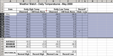
To sort the data on the new sheet:
- First you must indicate what data in the spreadsheet is to be sorted.
- Select rows 5 to 14 on the Sort by High Temp worksheet as
shown below (make sure to select the entire row so that all columns
are included).

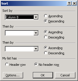
- On the Data menu, select Sort.
- The Sort options window appears. In this case, make sure to select
No header row, because we did not select the labels in row
4 as part of our highlighted data rows. We will sort on Column
B (observed daily high temperature) in Descending order
(highest values down to lowest values). Click OK to close this
window.

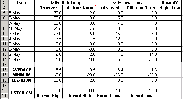
- The selected rows should now appear in a different order as shown
below. The date (8-May) with the largest Daily High appears first,
on down to the date with the smallest Daily High. None of the data
in rows 1 to 4, or 16 and beyond is altered. Nothing on any of the
other sheets in the workbook is altered either.

In Excel, you can set Protection options to prevent editing
(or even viewing) of all or parts of a workbook. This can be very useful
when you are sharing a spreadsheet with others or even to prevent yourself
from accidentally altering labels, formulas, etc. once they are all
completed.
In the following example, we will protect certain areas of the Main
worksheet from unintentional changes.
- Switch to the Main worksheet, if it is not already displayed.
- In Excel, it is necessary to set an option to unlock cells
that you still want to be able to change after a worksheet is protected.
By default every cell has its Locked property set to true.
In this example, let's say that we want to leave only the cells containing
the high and low temperature raw data open for editing after we (eventually)
protect the worksheet.
- Select the block of cells B5 to B14
- On the Format menu, select Cells.
- The Format Cells window appears. Click on the Protection
tab. Click in the box next to Locked to remove the check mark.
Click OK. You have now set the Locked property for these
cells to false.

- Select the block of cells D5 to D14 and do the same as above to
unlock them as well.
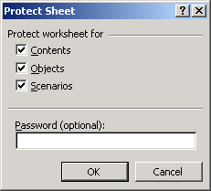
- On the Tools menu, point to Protection, and then click
Protect Sheet.
- The Protect Sheet window appears. Just leave the options
as they are and click OK.

- This provides a casual level of protection. (If you were really
more serious, for example if you wanted to prevent others from removing
worksheet protection, you could set a password. However, be aware
that if you assign a password, and forget it, you yourself will not
be able to alter the protected elements on the worksheet either.)
- If you have applied the protection options as per our instructions,
you should see the message below if you try to alter the contents
of any of the cells that remained locked on the Main sheet
(for example try to alter cells B16, F3 or E20). You should however
be able to modify the data in cells B5 to B14 or D5 to D14 (because
you unlocked those cells).

- If you want to change the Locked property of cells, the worksheet
must NOT be protected. Thus, once you have protected a sheet, you
must unprotect it before you can modify the Locked settings.
- To remove protection from a worksheet, display the worksheet,
then on the Tools menu, point to Protection, and then
click Unprotect Sheet. If a password was set you will be prompted
to enter the protection password for the worksheet. Passwords are
case sensitive. You must type the password exactly as it was created,
including uppercase and lowercase letters.
- Note: To move between unlocked cells on a protected worksheet,
click an unlocked cell, and then press the Tab key. The Tab
key is a handy way to let you cycle through the unlocked cells of
a sheet.
Title
Click here to return to the top of the page
| Page last updated on
October 31, 2002
|
|
|

